Human Resources Formulas and Functions in Excel (Plus Free Template)

Even with all the HR tech out there, spreadsheets are still everywhere. One recent report found 90% of organizations still rely on spreadsheets for some of their most vital business data. And while people analytics is clearly on HR’s agenda, many teams are still building the basics, with only 22% saying they’re very or extremely effective at getting value from people analytics today.

That’s where Excel earns its keep. It is not a replacement for your HRIS or advanced analytics tools, but for day-to-day tracking, quick checks, and ad hoc reporting, it’s hard to beat. For HR teams, that often means faster answers on headcount, hiring progress, time-to-fill, training completion, absence trends, and simple cost checks.

The better you get at Excel formulas and functions, the faster you can answer practical questions like “What changed?”, “Where are the outliers?”, and “Who needs attention?” You’ll also get more value from your HR systems by understanding what the dashboards are actually showing and by being able to validate the numbers behind them.

With that in mind, this guide shares some of the most common Human Resources formulas, tools, and functions in Excel, with examples you can use right away.

Contents
Working with dates
Formatting tables
Working with pivot tables
Common Human Resources formulas and metrics
HR Excel formulas practice template
ChatGPT prompts for HR in Excel

Working with dates

Let’s start with some commonly used date management functions.

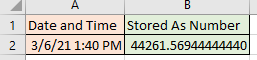
Excel stores dates as sequential serial numbers, starting with 1, with January 1, 1900, at 00:00 AM. March 16, 2021, is 44271 because it is the 44,271^st day since Excel’s date system starts.

Values less than a day are stored as decimal fractions.

Excel offers many ways to store, compare, and compute dates and times. There are 16 standard date formats, and custom formatting rules give you even more control over the display. To choose a format, right-click a cell (or range), select a date format, or choose Custom to see more options.

Before we start calculating dates, let’s see how we can enter today’s date—even if we don’t know what it is.

Using the TODAY() function

The TODAY function is a time-saving shortcut. It retrieves today’s date from your computer, so it updates automatically. Your worksheets update when you open or recalculate them.

If you need the current date and time, use NOW().

The function is handy for calculating things like age, time in service, or any case where the period you are using lacks a specific end. For example, if you want to calculate an employee’s age, you can subtract the employee’s birthdate from today. We start by formatting the column to display years instead of a serial number or date.

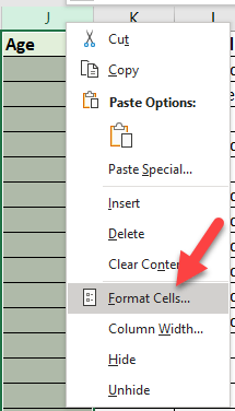
1. Right-click the Age column header. The Format Cells window will open.
2. Select Format Cells…
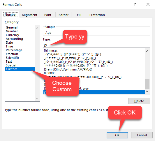
3. Custom opens the options; then you type “yy” (no quotes) in the Type field.
4. Click OK.

Finding the difference between two dates

Some of the things we do most frequently in HR measure the difference between two dates. We use those calculations for many reasons, including basics like the age of employees, time in service, benefits eligibility, pensions, and seniority.

There are many ways to calculate the difference. How you calculate them depends on your company’s practices, industry sector, and country or region.

We’ll give you four that we find useful and easy to use:

DATEDIF function

Excel DATEDIF returns the difference between two date values in years, months, or days. The DATEDIF (Date + Dif) function is a “compatibility” function from Lotus 1-2-3.

=DATEDIF(start_date, end_date, unit)

Unit Values

• “y” years
• “m” months
• “d” days
• “ym” months, ignoring years
• “yd” days, ignoring years and months

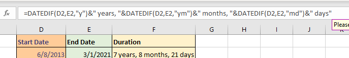
We can calculate years, months, and days using these formulas:

To give us this result:

Here is the same method using years, months, and days in a single cell:

DAYS360 function

Our Gregorian calendar makes things difficult for accountants, so they invented the 360-day year with 30 days in each month to create a tidy framework.

Although the Securities and Exchange Commission (SEC) does not accept it for formally published financial accounts, the 360-day Commercial Year is widely used to simplify interest calculations and internal valuations in business worldwide. Two accepted standards are the US (NASD) method and the European method.

The syntax is:

=DAYS360(start_date, end_date, method)

where method indicates a 360-day standard: FALSE for the US method and TRUE for the European method.

• In the US method, if a starting date is the last day of the month, it becomes the 30^th day of the month. If the ending date is the last day of a month and the starting date is earlier than the 30^th day of a month, the ending day is equal to the 1^st day of the next month. Otherwise, the ending day becomes equal to the 30^th of the same month.
• In the European method, starting and ending dates on the 31^st of the month equal the 30^th of the month. How’s that for tidy?

Caution:

Dates must be either derived from another function or entered using the DATE format:

DATE(yyyy,m,d) where DATE(2021,3,11) is March 11, 2021.

If start_date is after end_date, DATEDIF returns a #NUM! error.

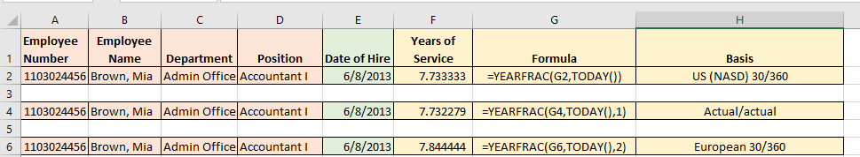
YEARFRAC function

If you want to calculate the difference between two dates as years and fractions of years, YEARFRAC will do it for you. The parameters for the function are the start date, end date, and basis, where the basis is 0 to 4:

Basis values

0 (or omitted)	US (NASD) 30/360
1	Actual/actual
2	Actual/360
3	Actual/365
4	European 30/360

Here’s the function itself:
  =YEARFRAC(start_date, end_date,[basis])

If you use YEARFRAC and the TODAY() function, it will always be correct.

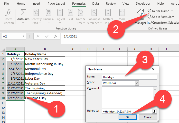
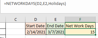
NETWORKDAYS function

NETWORKDAYS is a handy function for managing projects, schedules, or any time you need to calculate a span of workdays that includes holidays.

=NETWORKDAYS(start_date, end_date, holidays)

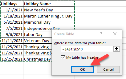
Here’s how we most often set up our holiday schedules. We create a worksheet named Holidays that contains the dates and names of holidays, then:

1. Select cell range $A$2:$A$10.
2. Click Define Name. The New Name window will open.
3. Type “Holidays” in the Name field.
4. Click OK.

Then, we can enter a NETWORKDAYS function anywhere in a workbook like this:

Formatting tables

Before we begin working with lookup formulas, let’s discuss how to format employee tables so your functions and procedures work consistently. Tables also reduce formula errors when rows get added, removed, or reordered, which is common in HR tracking sheets.

Every table should have a primary key. In Structured Query Language (SQL), a column or set of columns serves as a unique identifier. In Excel, we want the primary key to be a single column that identifies each data row.

If you work with employee information, the key is almost always the Employee ID. Placing it in the first (left-most) column in every worksheet that lists individual employees makes VLOOKUP, INDEX, MATCH, and INDEX-MATCH functions much easier to manage.

Format as Table function

We like to name our tables and arrays to make them easier to use. A quick way to do that is to use the Excel Format as Table function. 

1. Make sure your table is contiguous, with no gaps between columns or rows.
2. From the Home tab, click in the top left-most cell (A1).
3. Click on the Format as Table drop-down. The design panel will open.

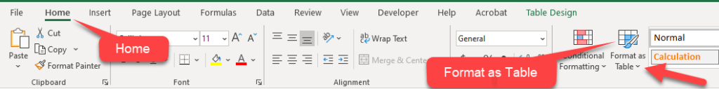
4. Click on the design you want. The table form will open, displaying the table range and indicating whether your table has headers. You will want headers, so if you don’t have them, go back and reformat your table.

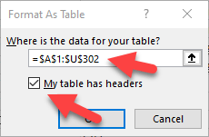
5. Click OK. Your table will be automatically formatted.
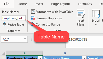
6. Give the table a name that makes sense to you. You can now use the table name in functions and formulas.

You can also use a keyboard shortcut to create tables.

1. Highlight your entire table.
2. Press Ctrl + T

You can then format it any way you like.

Filtering data

If you follow along in an Excel worksheet, you probably noticed that your tables automatically have filters. Filters are amazing time-savers when you want to slice and dice data. They can also be useful when you want to validate the data in a table.

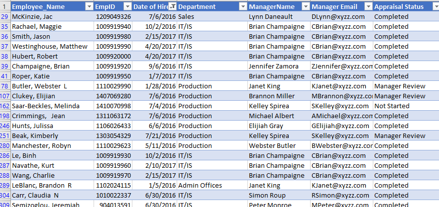
Suppose you needed to follow up on outstanding performance appraisals. You have a report listing all your employees and their appraisal status.

You could sort the worksheet by status and copy and paste the ones you need to follow up on, but it is easier to filter by the status you want to follow up on. In this example, we want to find all the appraisals that have not been started.

1. Click on the filter drop-down icon.

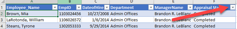
2. Clear the form by clicking on the (Select All) checkbox.

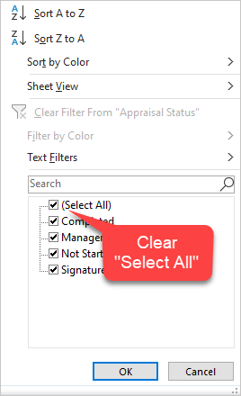
3. Select Not Started, then OK.

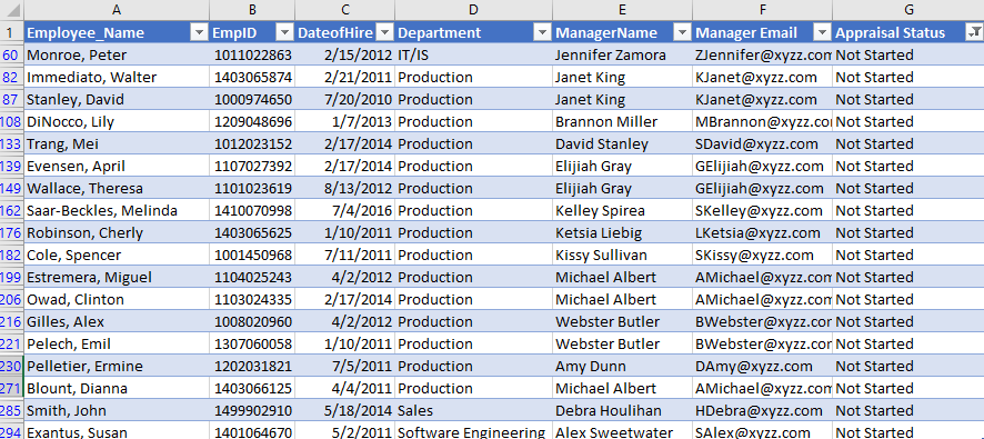
Here is what your filtered table would look like:

You can use multiple filters in various combinations based on the column’s data type. Number filters have many combinations, as do dates.

Now imagine you need a list of people hired between January 1, 2016, and December 31, 2018.

1. Click on the Date of Hire column filter. A list of filter options will open.
2. Select the Date Filters option. You now get a long list of filtering options.

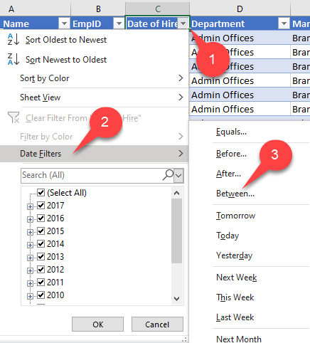
3. Select Between and fill in the date parameters.

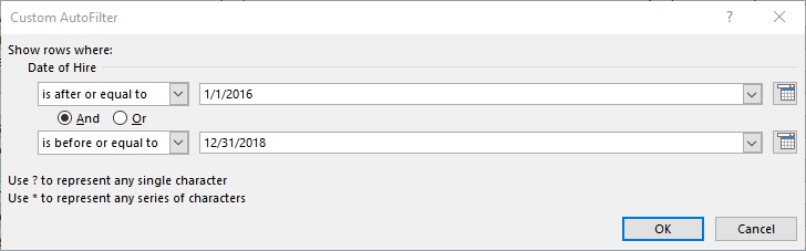
Your report is ready:

Working with pivot tables

Of all the features, functions, and tools in Excel, pivot tables are among the most useful. They are dynamic summary reports you generate from a database, a table in a worksheet, an external data file, or an external database.

Check out our video to find out how you can use Pivot Tables for Excel!

PivotTables let you turn any data source into a flexible summary report in a few clicks. You can then slice and dice, summarize and combine, and manipulate data in just about any way you can imagine. This is a practical way to summarize trends like turnover reasons, absence categories, or training completion by department.

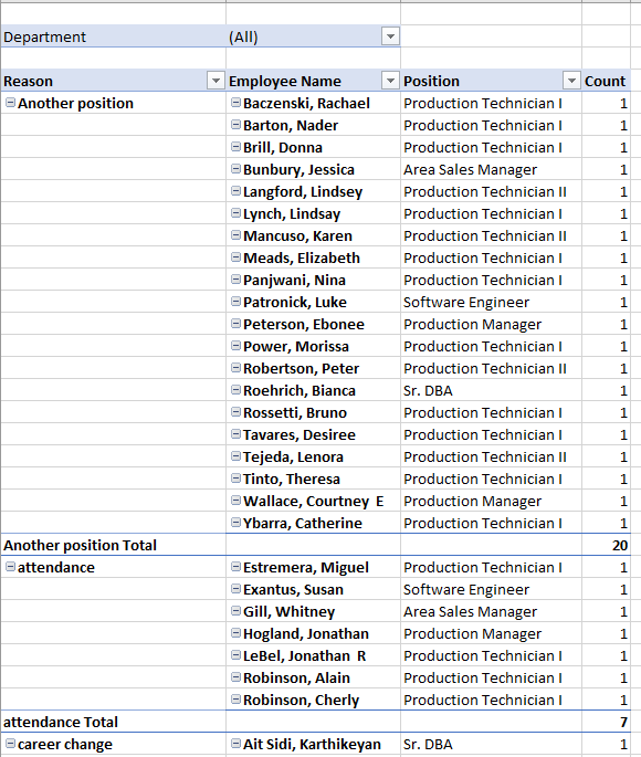
We will show you how to create a termination reasons report by department. You can get a copy of the dataset we are using on Kaggle (mirror).

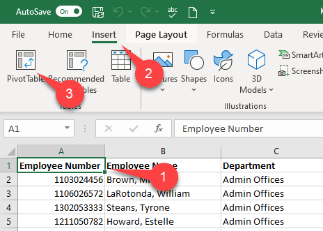
Here’s how to create a report from any worksheet:

1. First, we click in the top-left cell (A1) in a contiguous table of employee data. A good data sample will have the employee number, a value unique to each individual, in column A.
2. We click on the Insert menu.
3. Then, we click on the PivotTable icon. The Create PivotTable form will open.

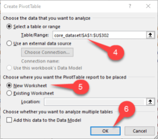
4.  Excel automatically selects our entire table of data.
5. We select New Worksheet to tell Excel where to put the table.
6. Then, click OK.

7. A new tab will open with a blank pivot table on the left and the PivotTable Fields form on the right. Do housekeeping first by renaming the tab so you can find it later.

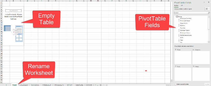
8. In the PivotTable Fields form, drag Date of Termination to the Values section, giving us a numerical value for the table to count.

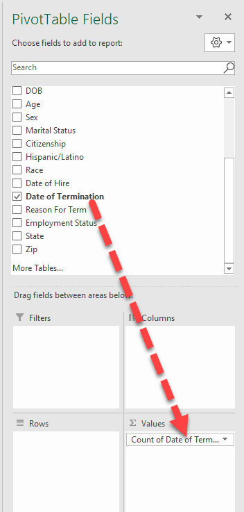
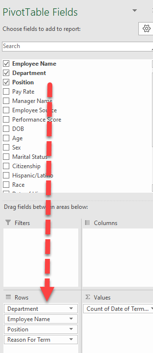
9. We also drag Department, Employee Name, Position, and Date of Term to the Rows section.

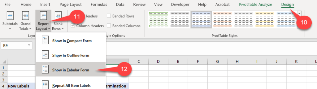
At this point, the table will start to take shape, but it may look a bit messy at first. We’ll fix that now.

10. Click anywhere in the table, then click on Design. The design menu appears.
11. Click on Report Layout.
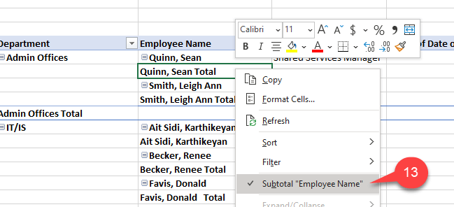
12. We click on Show in Tabular Form. It starts to make sense, but we don’t need a subtotal in the Employee Name column.

13. Right-click in the Employee Name column and click on Subtotal “Employee Name” to uncheck it. We do the same with the Position column.

We now have a neat table showing the number of terminations and reasons for each department.

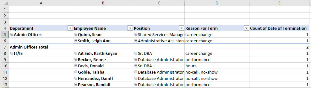
There is just a little cleanup to do. Some of the column names are a bit long and confusing. We can enter new names directly into the column headers.

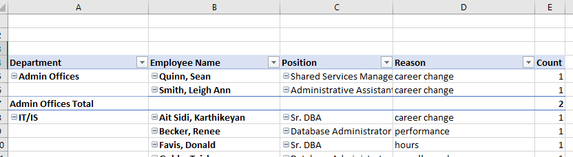
One more thing:

Let us explain why this tool is called a pivot table.

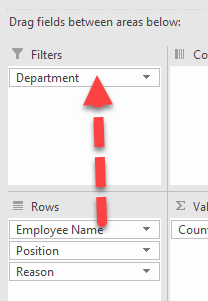
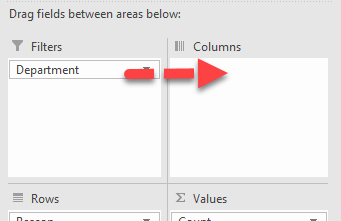
In the PivotTable Fields form, we select the Department field and drag it to the Filters section to pivot it from a row field to a filter, allowing us to change the report to show a single department or any combination.

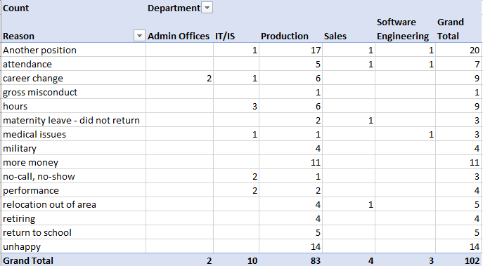
Now, we’ll try another pivot. We right-click on the Reason field, hover on Move, then click on Move “Reason” to Beginning.

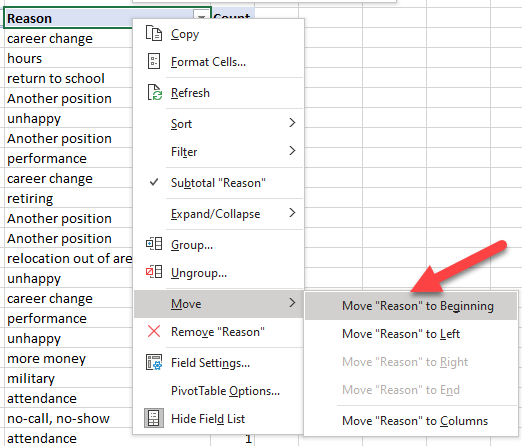
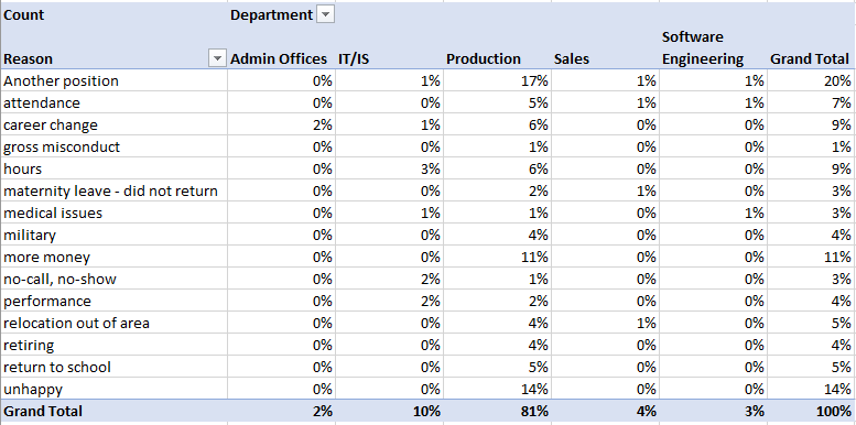
We now have a report on reasons for termination.

Pivot table columns

If we wanted to see the reasons for the terminations summarized for each department, we could use columns to show the departments.

Let’s remove the report’s names and positions to reduce clutter, then drag the department to the Columns section. We now have a summary report, but it’s not very useful.

Let’s change the way we summarize the data. Right-click in the Grand Total cell and select Show Values As, then % of Grand Total.

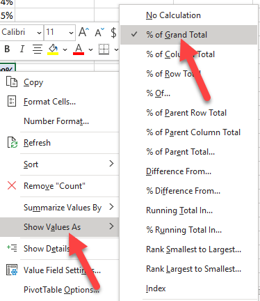
After we use the Grand Total cell to format the numbers as a Percent with no decimals, we have a report that tells us something about where we might need an intervention.

We’ve given you only a quick introduction to the power of pivot tables. We hope it whets your appetite to learn more.

Common Human Resources formulas and metrics

Excel has hundreds of formulas that can help HR work faster, but a few stand out because they support the HR metrics that come up again and again in reporting and decision-making.

Cost of benefits and employee programs

Calculating benefits (including employee programs) helps you understand what you spend beyond base pay and build a more complete view of employee cost. These numbers also feed into other internal metrics and budgeting conversations.

Benefits costs per employee

Benefits cost per employee is the total spend on benefits and employee programs divided by the average number of employees.

“benefits_cost = total_cost_of_benefits_and_programs ÷ average_number_of_employees

This helps you compare benefit spend across teams or time periods. You can calculate it per month, quarter, or year for comparisons over time.”

Benefits and programs as a percent of pay

This ratio shows benefits cost relative to payroll.

benefits_ratio = cost_of_benefits ÷ total_pay 

This makes it easier to benchmark benefit load against payroll.

Total employee cost

Once you have the benefits ratio, you can estimate total employee cost (pay plus benefits) like this:

total_employee_cost = (1 + benefits_ratio) × total_pay 

This gives you a quick ‘all-in’ cost estimate for budgeting and scenario planning.

Revenue

In HR, we sometimes get so focused on cost that we forget to show our business impact. We recommend partnering with managers and leaders throughout the business to answer the most important questions when making a change or implementing an intervention. They are: What moved? By how much?

Revenue per employee

Revenue per employee is a simple way to connect people data with business performance. Pull top-line revenue from your financial reports and divide it by the average number of employees.

revenue_per_employee = top_line_revenue ÷ average_number_of_employees

Use average headcount for the period so you don’t overstate or understate the metric when hiring ramps up or down.”

Tenure and turnover

Employee tenure

You can calculate tenure using hire date and today’s date, then take the average across employees.

1. Format your list as a table.
2. Create a new column next to Hire Date named Tenure. Then, enter the formula in the top cell.
   =yearfrac([hire_date],today())
3. In the Number menu group, format the value using the comma icon (Accounting format).
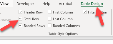
4. In the Table Design tab, check the Total Row checkbox. The view will jump to the bottom row.

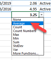
5. In the Tenure column, select the Average function.

Talent acquisition metrics

Recruiting costs are a critical business metric. You need to know how much time it takes and what it costs to hire talent. Then, you can compare those costs against what you spend on employee engagement, retention, and development.

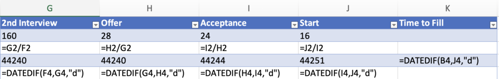
Time to fill a vacancy

Time to fill measures the number of workdays it takes to source, select, and hire. When the pipeline slows down, costs can climb quickly: overtime, workload strain, and delays to business outcomes.

An inefficient pipeline can cause costs to grow out of control, and the impact is much more than the cost of operating the recruiting function. Your people must cover the vacancy, and you may incur overtime costs. There will be additional stress on the people who cover it.

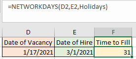
First, we define a table named “Holidays” to use as a NETWORKDAYS function parameter. 

Cost per hire

Cost per hire includes covering the vacancy, the direct costs of advertising and hiring, and the cost of managers and recruiters in the process. Here’s a sample breakdown of the talent acquisition cost, along with the respective HR formulas.

Yield ratio

Yield ratio helps you understand efficiency at each stage of the pipeline. It measures how many applicants move from one step to the next.

yield_ratio = applicants_at_step ÷ applicants_at_previous_step

Hiring velocity

Time to fill and hiring velocity are not the same. Time to fill is the total time required for the process, whereas hiring velocity looks at the speed of movement between steps. This matters because slowdowns can lead to candidate drop-off (including ghosting). Track velocity alongside yield ratio to spot where the process stalls.

You can track velocity along with your yield ratio. Here are the formulas.

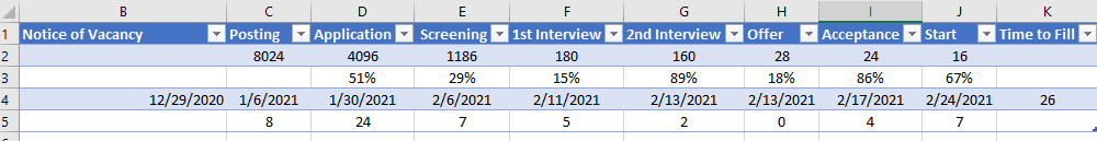
And the result. We calculated the total time to fill in the last column.

HR Excel formulas practice template

We’ve created a free, editable HR Excel template so you can practice some of the formulas in this guide without building a dataset from scratch. It comes with a sample employee table and pre-filled formula examples you can reuse in your own reporting.

ChatGPT prompts for HR in Excel

If you use Excel for day-to-day HR tracking and quick reporting, ChatGPT can help you get to the right formula faster. Below are a few examples from our ChatGPT for Excel one-pager, split into beginner and advanced prompts. These are just a sample, so if you want the full list of prompts and outputs, you can download a handy PDF right below this section.

Beginner prompts

Count values (candidate pipeline)

• Prompt: “In my Excel sheet, candidate status is in column D. Write a formula to count how many candidates have status ‘Hired’.”
• Output: =COUNTIF(D:D, "Hired")
• What it does: Counts how many times “Hired” shows up in column D.

Combine data from multiple cells into a single cell

• Prompt: “First name is in column B and last name in column C. Write a formula to combine them into full names.”
• Output: =CONCATENATE(B2, " ", C2) or =B2 & " " & C2
• What it does: Joins the first and last name into one full name, with a space in between.

Check for missing values

• Prompt: “Bonus data is in column F. Write a formula to return ‘Missing’ if empty, ‘OK’ if filled.”
• Output: =IF(ISBLANK(F2), "Missing", "OK")
• What it does: Flags blank bonus cells so you can spot missing data fast.

Advanced prompts

Calculate averages

• Prompt: “Salary is in column E, department in D. Write a formula to get average salary for HR only.”
• Output: =AVERAGEIFS(E:E, D:D, "HR")
• What it does: Averages salaries only for rows where the department is HR.

Rank values

• Prompt: “Performance scores are in column G. Write a formula to rank each employee.”
• Output: =RANK.EQ(G2, G:G, 0)
• What it does: Ranks each score against the full list, highest score gets rank 1.

Look up with XLOOKUP

• Prompt: “ID is in column A, department in D. Write an XLOOKUP formula to find the department based on ID in A2.”
• Output: =XLOOKUP(A2, A:A, D:D)
• What it does: Finds the employee ID in column A and returns the matching department from column D.

Over to you

Excel formulas are not just spreadsheet shortcuts. They’re your starting point for faster analysis, better decisions, and more strategic conversations across your organization. Use them to explore your data with confidence, spot patterns, and back your HR instincts with numbers.

The more you apply them to your real-world challenges—whether that’s tracking turnover, identifying high performers, or analyzing training impact—the more confident and capable you’ll become in using Excel to drive smarter HR decisions.